Visual text Analytics with python
Due to the flourish of internet and accessibility of technology incredible platforms like social media, forums, etc have been created for knowledge sharing. Exchanging ideas is not confined to a geographical area. Due to this volume and variety of content is generated in the form of images, video, text, etc. The amount of information is so much that it’s unmanageable to perceive it in bounded time, in such times area of text analytics has got the attention of people in the field of linguistics, business, etc. The goal of the post is to summarize few of the visual text analytical techniques that could help you in your initial phase of text mining or help you create a new feature for creating machine learning model. I will describe few online and offline tools that you could use to help you get started. By offline tools, I mean using python based software packages to created visualization and text pre-processing. Online tools will be web-browser based applications to which just have to paste the text or upload the text file to visualise the results.
#Visual Text Analytics
Exploratory text analysis can help us to get the gist of the text data. I am going to use python for the code example and for text processing. For text processing and text corpus I will be using nltk package and for visualization matplotlib package. There are also other packages that we will use as we progress.
-
WordCloud: one of the simplest visualization technique which is a type of word frequency visualization. The size of the word in the image is bigger for more frequent word and smaller for less frequent word. This type of visualization can be of help in initial query formation. There are some drawbacks like the longer word may occupy more space giving the impression of the frequent word than it actually is. It may not help us to compare two frequent words about their relationship can be misleading sometimes even if using two words together may make sense. Frequent words may not be meaningful. For generating word cloud I am going to use wordcloud package you can install the package from pip. Below is the code to generate cloud. Text dataset used is the US presidential inaugural addresses which are part of nltk.corpus package.
1
2
3
4
5
6
7
8
9
10
# import the dataset
from nltk.corpus import inaugural
# extract the datataset in raw format, you can also extract it in other formats as well
text = inaugural.raw()
wordcloud = WordCloud(max_font_size=60).generate(text)
plt.figure(figsize=(16,12))
# plot wordcloud in matplotlib
plt.imshow(wordcloud, interpolation="bilinear")
plt.axis("off")
plt.show()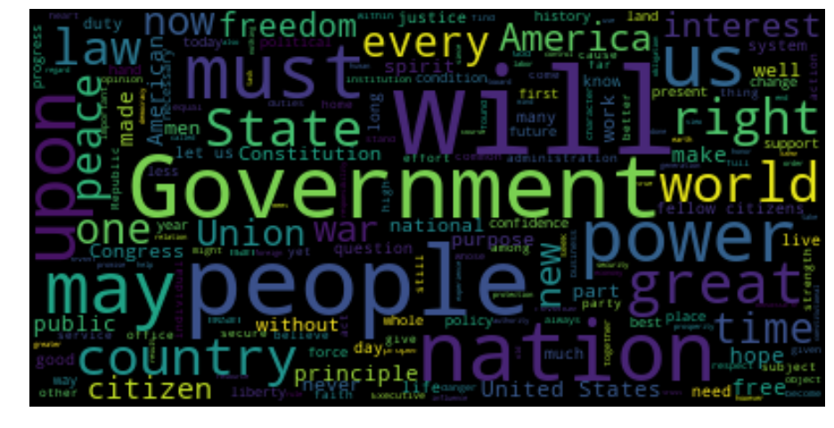
-
Lexical dispersion plot: this is the plot of a word vs the offset of the word in the text corpus.The y-axis represents the word. Each word has a strip representing entire text in terms of offset, and a mark on the strip indicates the occurrence of the word at that offset, a strip is an x-axis. The positional information can indicate the focus of discussion in the text. So if you observe the plot below the words America, democracy and freedom occur more often at the end of the speeches and words like duties and some words have somewhat uniform distribution in the middle. This way we can conclude that as the speech started the focus was on duties but then focus shifted to America, democracy and freedom. Below is the code to reproduce the plot.
1
2
3
4
from nltk.book import text4 as inaugural_speeches
plt.figure(figsize=(16,5))
topics = ['citizens', 'democracy', 'freedom', 'duties', 'America','principle','people', 'Government']
inaugural_speeches.dispersion_plot(topics)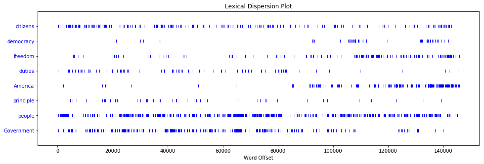
-
Frequency distribution plot: this plot tries to communicate the frequency of the vocabulary in the text. Frequency distribution plot is word vs the frequency of the word. The frequency of the word can help us understand the topic of the corpus. Different genre of text can have a different set of frequent words, for example, If we have news corpus then sports news may have a different set of frequent words as compared to news related to politics, nltk has FreqDist class that helps to create a frequency distribution of the text corpus. The code below will find 5 most and least frequent words.
1
2
3
4
5
6
7
8
9
10
11
from nltk.corpus import brown
topics = ['government', 'news', 'religion','adventure','hobbies']
for topic in topics:
# filter out stopwords and punctuation mark and only create array of words
words = [word for word in brown.words(categories=topic)
if word.lower() not in stop_words and word.isalpha() ]
freqdist = nltk.FreqDist(words)
# print 5 most frequent words
print(topic,'more :', ' , '.join([ word.lower() for word, count in freqdist.most_common(5)]))
# print 5 least frequent words
print(topic,'less :', ' , '.join([ word.lower() for word, count in freqdist.most_common()[-5:]]))output for above code is presented in the table format below. It will be surprising to see that in least frequent table words belonging to a category of text corpus are more informative compared to the words found in the most frequent table which is the core idea behind TF-IDF algorithm. Most frequent words convey little information about text compared to less frequent words.
Most 5 Frequently occurring words
government news religion adventure hobbies year said god said one states would world would may united one one man time may last may back two would two new one first Least 5 Frequently occurring words
government news religion adventure hobbies wage macphail habitable sprinted majestic irregular descendants reckless rug draft truest jointly mission thundered gourmets designers amending descendants meek fastenings qualities plaza suppose jointly fears The code below will plot frequency distribution for a government text, you can change the genre to see distribution for a different genre like try humor, new, etc.
1
2
3
4
5
6
# get all words for government corpus
corpus_genre = 'government'
words = [word for word in brown.words(categories=corpus_genre) if word.lower() not in stop_words and word.isalpha() ]
freqdist = nltk.FreqDist(words)
plt.figure(figsize=(16,5))
freqdist.plot(50)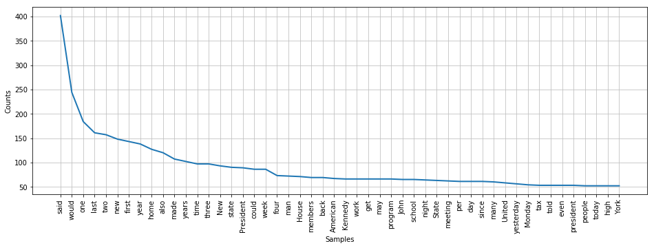
-
Lexical diversity dispersion plot: lexical diversity lets us what is the percentage of the unique words in the text corpus for example if there are 100 words in the corpus and there are only 20 unique words then lexical diversity is 20/100=0.2. The formula for calculating lexical diversity is as below :
$$ \text{Lexical diversity(LD)}= \frac{\text{Number of unique words}}{\text{Number of words}} $$
Below is the python function to calculate the lexical diversity1
2
3
4
5
6
7
8
9
10
11
12
13
14
15
16
17
18
19def lexical_diversity(text):
return round(len(set(text)) / len(text),2)
def get_brown_corpus_words(category, include_stop_words=False):
'''helper method to get word array for a particular category
of brown corpus which may/may not include the stopwords that can be toggled
with the include_stop_words flag in the function parameter'''
if include_stop_words:
words = [word.lower() for word in brown.words(categories=category) if word.isalpha() ]
else:
words = [word.lower() for word in brown.words(categories=category)
if word.lower() not in stop_words and word.isalpha() ]
return words
# calculate and print lexical diversity for each genre of the brown corpus
for genre in brown.categories():
lex_div_with_stop = lexical_diversity(get_brown_corpus_words(genre, True))
lex_div = lexical_diversity(get_brown_corpus_words(genre, False))
print(genre ,lex_div , lex_div_with_stop)The table below summarizing the result of the above code, humor category seems to have most lexical diversity followed by science fiction, government genre has the least diversity. If we remove the stopwords then the metric seems to change which is shown in the rightmost column in the table, metrics seems to get almost half.
stopwords are extremely common words that have very little or of no valuable information like the, are, as, by, etc.
Genre LD (with stopwords) LD (w/o stopwords) Humor 0.49 0.25 Science Fiction 0.47 0.24 Reviews 0.39 0.21 Religion 0.32 0.16 Editorial 0.29 0.16 Fiction 0.28 0.14 Adventure 0.26 0.13 Mystery 0.26 0.13 Romance 0.26 0.13 Hobbies 0.25 0.13 News 0.24 0.13 Lore 0.24 0.13 Government 0.20 0.11 Belles Lettres 0.20 0.10 Learned 0.16 0.09 It would also be interesting to see how to lexical diversity changes in the corpus. To visualise this we can divide a text corpus into small chunks and calculate the diversity for that chuck and plot it. Corpus can be divided by sentence or we can consider each paragraph as chunks but for sake of simplicity we can consider a batch of 1000 words as a chunk and plot its lexical diversity. So x-axis is the chunk offset and y-axis is the lexical diversity of that chunk. Below is the code to plot lexical diversity distribution for different genre of brown text corpus
1
2
3
4
5
6
7
8plt.figure(figsize=(16,8))
for cat in brown.categories():
plot_array = lexical_array(cat)
plt.plot(np.arange(0,len(plot_array))*5000,plot_array,label=cat)
plt.legend()
plt.xlabel('Word offset')
plt.ylabel('Lexical diversity')
plt.show()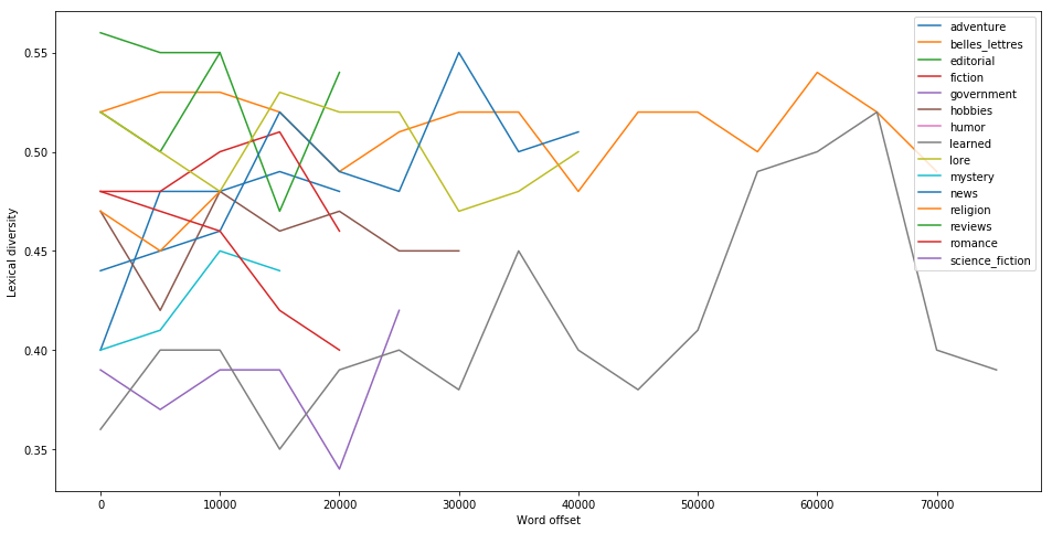
Observing the plot we can conclude that some genre of text starts with less diversity and diversity increases as the corpus offset increases like learned. But for some genre, the lexical distribution is high on an average example is belles_letters vs learned category.
-
Word length distribution plot: This plot is word length on x-axis vs number of words of that length on the y-axis. This plot helps to visualise the composition of different word length in the text corpus. Below is the code the achieve this
1
2
3
4
5
6
7
cfd = nltk.ConditionalFreqDist(
(genre, len(word))
for genre in brown.categories()
for word in get_brown_corpus_words(genre))
plt.figure(figsize=(16,8))
cfd.plot()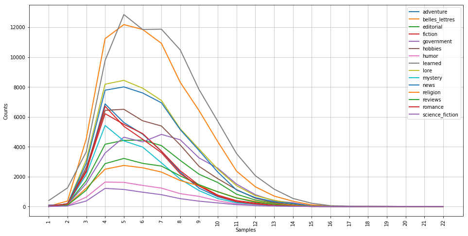
-
N-gram frequency distribution plot: n-grams is the continuous sequences of n words that occur very often for example for n=2 we are looking for 2 words that occur very often together like New York, Butter milk, etc. such pair of words are also called bigram, for n=3 its called trigram and so on. N-gram distribution plot tries to visualise distribution n-grams for different value of n, for this example, we consider n from 1 to 5. In the plot, x-axis has the different value of n and y-axis has the number of time n-gram sequence has occurred. Below is the code to plot the distribution plot.
1
2
3
4
5
6
7
8
9
10
11
from nltk.util import ngrams
plt.figure(figsize=(16,8))
for genre in brown.categories():
sol = []
for i in range(1,6):
count = 0
fdist = nltk.FreqDist(ngrams(get_brown_corpus_words(genre), i))
sol.append(len([cnt for ng,cnt in fdist.most_common() if cnt > 1]))
plt.plot(np.arange(1,6), sol, label=genre)
plt.legend()
plt.show()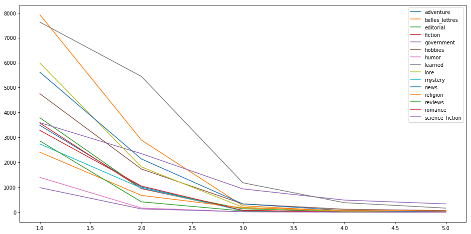
#Online tools
This section of the post is for those people who might feel lazy or just don’t want to code to get the work done, you could use some of the tools available online which require no coding skills. You just have to paste the text or upload the file to get nice visualization. Below is the list of few tools that I found to be useful.
- Voyant: this app produces some of the above plots on a nice web dashboards. The plots which could be found are wordcloud, trend graph, etc. If you click on the word in the reader tab you will able to see all the sentence in which the word appears which can be very helpful to do some query based on words. There are also other metrics to explore, I would suggest you to explore the dashboard in detail.
- Visualize text as a network : This tool visualises text as a graph, the details of the algorithms on how to produce the graph is published inthis paper. If you click on one node it will highlight all connected nodes. The words which we see on the nodes are called concepts and the concepts which are related are connected by edges.
- Google n-gram viewer: Google has a very big corpus of books data which could be queried with this tool. What this tool give is the tread of words used in the books written in English and publish in the United States, for example, you can query trends in three n-grams from 1950 to 2000: “health care” (a 2-gram or bigram), “healthy” (a 1-gram or unigram), and “child care” (another bigram). In the chart y-axis shows all the bigrams word contained in the books, what percentage of them are “health care” or “child care”? Of all the unigrams, what percentage of them are “healthy”? you can see how the use of the words have changed over time if you are querying multiple words then you can compare their trends. There few advanced features of the Ngram Viewer, for those who want to dig a little deeper into phrase usage: wildcard search, inflection search, case-insensitive search, part-of-speech tags and n-gram compositions, more info on these features can be found on this link.
- ANNIS: is an open source, web browser-based search and visualization architecture for complex multi-layer linguistic corpora with diverse types of annotation. ANNIS, which stands for ANNotation of Information Structure. ANNIS addresses the need to concurrently annotate, query and visualise data from such varied areas as syntax, semantics, morphology, prosody, referentiality, lexis and more. For projects working with spoken language, support for audio/video annotations is also required. You can query large-scale dataset as ANNIS store data in Postgres which faster as compared to other storage formats like XML.
- TokenX: is a free and open-source cross-platform Unicode & XML based text/corpus analysis environment and graphical client, supporting Windows, Linux and Mac OS X. It can also be used online as a J2EE standard compliant web portal (GWT based) with access control built in.
#Conclusion
Exploratory text analytics can be really simple as we saw, some basic visualization can help you to get a good understanding of the text corpus and also some of the metrics discussed above can help you to compare different text corpus in your dataset. We also discussed some online tools which can help you to dig deeper you can try analysing some of the datasets whose link I have posted in below play around which these tools.